How It Started

I was only acquainted with cohort analysis but thanks to Renat Alimbekov, I got introduced to the topic with practice. Renat is a Deep Learning Scientist with a telegram channel and a blog, as well as a mentor at Yandex.Praktikum. I had a different mentor during my studies but I’ve been following Renat’s telegram channel and noticed that he started giving typical data science assignments. So I accepted this challenge and started with this project. His solution can be found here.

Introduction

In the task we’re given a dataset of Brazilian Ecommerce by Olist¹, the two tables to merge (olist_orders_dataset.csv and olist_order_payments_dataset.csv), and two questions:

1. How many orders on average, and how much do all cohorts make in the first year?
2. Compare any of the two cohorts by revenue and number of orders

It was a late night last Thursday, I gave it a try before going to sleep. When I was solving it, the words “in the first year” made me jump over to the next question cause it was time to sleep. I decided to see what I would get in the second question, solved it in a different way (from what one will see below, also I first used a different cohort column) and tagged Renat in a tweet. He gave me some feedback so I felt encouraged to get back to the task. In one of the following nights I wrote a few ideas of how to approach the first question just before falling asleep (see the time in the screenshot).

¹ Olist operates an online e-commerce site for sellers, that connects merchants and their products to main marketplaces.

My Solution

Merging the tables

order_payment = orders.merge(payments, how='inner', on='order_id')

The column we use to define cohorts:

cohort_column = 'order_purchase_timestamp'

So I wanted to find the gap between the first and last order, then select the orders made within 365 days after the first order was made. I saved the first and last orders:

order_payment[cohort_column] = pd.to_datetime(order_payment[cohort_column])
first_orders = order_payment.pivot_table(index='customer_id', values=cohort_column, aggfunc={cohort_column:'first'}).reset_index()
last_orders = order_payment.pivot_table(index='customer_id', values=cohort_column, aggfunc={cohort_column:'last'}).reset_index()
first_orders.columns = ['customer_id', 'first_order']
last_orders.columns = ['customer_id', 'last_order']

Let’s now calculate the difference between the first order and the last order.

day_diff = first_orders.merge(last_orders.set_index('customer_id'), on='customer_id')
day_diff['day_diff'] = ((day_diff['last_order'] - day_diff['first_order']).astype("timedelta64[D]")).astype('int')
day_diff.head(3)

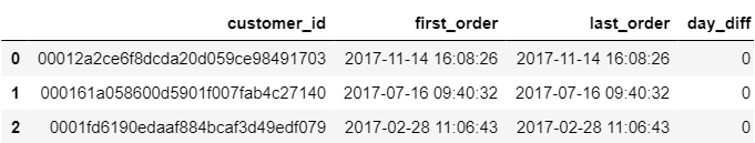
Okay, the gap has been calculated.

print('Number of customers whose latest order was made in other days after the first order is', (day_diff['day_diff'] > 0).sum())

Number of customers whose latest order was made in other days after the first order is 0

However this is weird. Since none of these so-called next orders was made at a different point in time, I believe those were other items in a cart that were registered as different orders. We see that if we just drop the payment details and calculate duplicates (i.e. multiple orders made by one customer), the time the purchase was made in remains the same for the same customers:

same_time_customer_orders = order_payment.drop(['order_id','payment_sequential','payment_type','payment_installments', 'payment_value'], axis=1).duplicated(keep=False).sum()
print("Total number of multiple orders made by the same customers at one time in time for each customer is", same_time_customer_orders)

Total number of multiple orders made by the same customers at one time in time for each customer is 7407

One would expect that a customer is coming back but considering the previous discovery, I’d assume that these were one-time purchases of multiple items registered as multiple orders.

Since the purchase time is never different that makes it simpler and there’s no need to select orders made within 365 days after the first order of every customer. I can now move on to the cohort analysis questions set by Renat.

all_orders = len(orders)
all_orders

99441

There’s a total of 99441 orders.

• How many orders on average, and how much do all cohorts make in the first year?

I’m creating a pivot table to rearrange the dataset by customer and order_status with the columns that I need for analysis. Will explain the reason why I need ‘order_status’ column in a few moments.

orders = order_payment.pivot_table(index=['customer_id', 'order_status'], values=[cohort_column, 'payment_value', 'order_id'], aggfunc={cohort_column:'min', 'payment_value': 'sum', 'order_id': 'count'}).reset_index()

orders.columns = ['customer_id', 'order_status', 'order_count', 'order_date', 'payment_value']
orders['order_year'] = orders['order_date'].dt.year
orders['order_month'] = orders['order_date'].dt.month

Orders have different statuses.

orders['order_status'].unique().tolist()

['delivered',
 'unavailable',
 'processing',
 'shipped',
 'canceled',
 'invoiced',
 'created',
 'approved']

orders = orders[(orders['order_status'] != 'unavailable') & (orders['order_status'] != 'canceled')]

Let’s choose all orders except the ones where status is unavailable or canceled. The shop has to return the payment for these orders back to customers, so this probably shouldn’t count.

paid_orders = len(orders)
paid_orders

98206

paid_orders_percent = paid_orders / all_orders

0.9875905068382944

There are 98206 paid orders where some of the payments might be refunded (either due to being unavailable or canceled) but weren’t at the moment of data extraction from the database. One can also see that only ~1.24% (1 - paid_orders_percent) of orders turned to be somewhat problematic so far. Within each cohort I’ll calculate the number of customers, total orders and payments by making a pivot table.

df = orders.pivot_table(index = ['order_year', 'order_month'], values=['customer_id','payment_value', 'order_count'], aggfunc={'customer_id': 'count', 'order_count':'sum', 'payment_value':'sum'}).reset_index()

df.columns = ['order_year', 'order_month', 'customer_count', 'order_count', 'payment_value'] #changing column names

Concatenating the columns to have a clear name of each cohort.

df["cohort"] = df["order_year"].astype(str) + "-" + df["order_month"].astype(str)

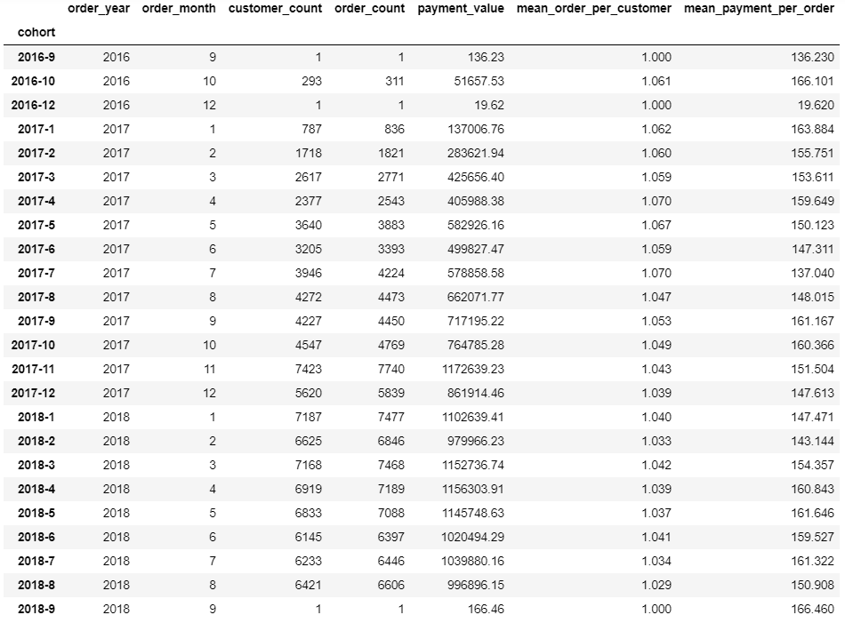
Calculating the average amount of orders per customer and average payment amount per order, rounded to 3 decimals.

df['mean_order_per_customer'] = round(df['order_count'] / df['customer_count'], 3)
df['mean_payment_per_order'] = round(df['payment_value'] / df['order_count'], 3)

df = df.set_index('cohort')
df

import matplotlib.pyplot as plt

plt.figure(figsize=(12,7))
plt.plot(df['payment_value'])
plt.xticks(rotation='45')
plt.title('Total Payments by Cohort', fontsize=14)
plt.xlabel('Cohort', fontsize=13)
plt.ylabel('Total Payments', fontsize=13)
plt.show()

Clearly, there has been a growth with a peak in a cohort of November 2017, however it’s worth a remark that data are missing for the following months 2016-9, 2016-12, and 2018-9.

plt.figure(figsize=(12,7))
plt.plot(df['mean_order_per_customer'])
plt.xticks(rotation='45')
plt.title('Mean Order Count Per Customer by Cohort', fontsize=14)
plt.xlabel('Cohort', fontsize=13)
plt.ylabel('Mean Order Count Per Customer', fontsize=13)
plt.show()

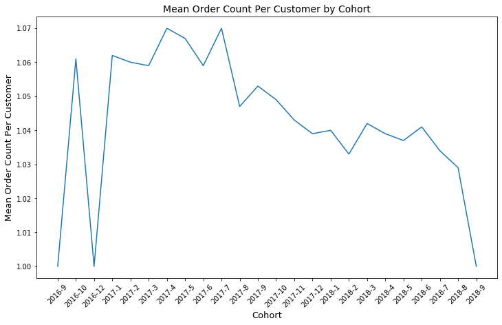
The chart shows a decrease in an average number of orders per customer after July 2017. It didn’t increase afterwards. That’s interesting, it feels like ecommerce shops chose a different growth strategy to concentrate on attracting new customers, though we don’t know the real reason.

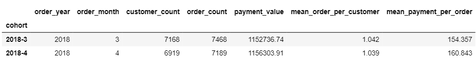
• Compare any of the two cohorts by revenue and a number of orders

selected_cohorts = df.loc[['2018-3', '2018-4']]
selected_cohorts

selected_cohorts.iloc[1] - selected_cohorts.iloc[0]

order_year                    0.000
order_month                   1.000
customer_count             -249.000
order_count                -279.000
payment_value              3567.170
mean_order_per_customer      -0.003
mean_payment_per_order        6.486
dtype: float64

The two cohorts are of interest to me because of comparable payment values while the mean order per customer is smaller by 0.003 in the second (2018-4), on average these customers paid more by around 6.5 currency units. Perhaps it’s worth studying the profile of those particular well paying customers in detail for advertisement. :)

Conclusion

One can clearly see a positive correlation between customer base growth and payment values. Mean payment per order didn’t go below 150 during the period from March 2018 to August 2018. However, it would be interesting to see if it started decreasing which is impossible due to a lack of data. Though maybe it would be great to come back to doing the same thing as in that 6 month period.